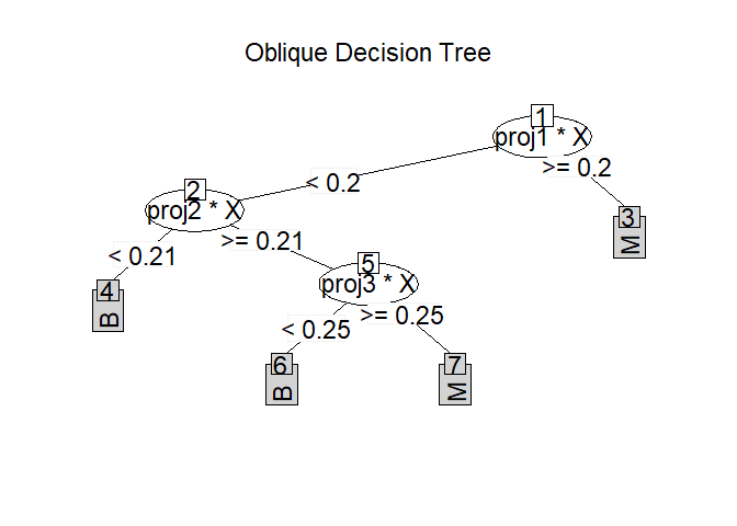
Find the optimal projection using various projectin pursuit models.
Arguments
- X
An n by d numeric matrix (preferable) or data frame.
- y
A response vector of length n.
- model
Model for projection pursuit.
"PPR"(default): projection projection regression from
ppr. When y is a category label, it is expanded to K binary features."Log": logistic based on
nnet."Rand": The random projection generated from \(\{-1, 1\}\). The following models can only be used for classification, i.e. the
splitmust be ”entropy” or 'gini'."LDA", "PDA", "Lr", "GINI", and "ENTROPY" from library
PPtreeViz.The following models based on
Pursuit."holes": Holes index
"cm": Central Mass index
"holes": Holes index
"friedmantukey": Friedman Tukey index
"legendre": Legendre index
"laguerrefourier": Laguerre Fourier index
"hermite": Hermite index
"naturalhermite": Natural Hermite index
"kurtosismax": Maximum kurtosis index
"kurtosismin": Minimum kurtosis index
"moment": Moment index
"mf": MF index
"chi": Chi-square index
- split
The criterion used for splitting the variable. 'gini': gini impurity index (classification, default), 'entropy': information gain (classification) or 'mse': mean square error (regression).
- weights
Vector of non-negative observational weights; fractional weights are allowed (default NULL).
- ...
optional parameters to be passed to the low level function.
References
Friedman, J. H., & Stuetzle, W. (1981). Projection pursuit regression. Journal of the American statistical Association, 76(376), 817-823.
Ripley, B. D. (1996) Pattern Recognition and Neural Networks. Cambridge.
Lee, YD, Cook, D., Park JW, and Lee, EK(2013) PPtree: Projection Pursuit Classification Tree, Electronic Journal of Statistics, 7:1369-1386.
Cook, D., Buja, A., Lee, E. K., & Wickham, H. (2008). Grand tours, projection pursuit guided tours, and manual controls. In Handbook of data visualization (pp. 295-314). Springer, Berlin, Heidelberg.
Examples
# classification
data(seeds)
(PP <- PPO(seeds[, 1:7], seeds[, 8], model = "Log", split = "entropy"))
#> [1]  -2.309383   2.847194  31.625381  35.243198   3.104818  -1.524764 -36.500103
(PP <- PPO(seeds[, 1:7], seeds[, 8], model = "PPR", split = "entropy"))
#> [1] -0.04663995 -0.01700724 -0.92771564 -0.23227466  0.20425324  0.01478790
#> [7]  0.20245882
(PP <- PPO(seeds[, 1:7], seeds[, 8], model = "LDA", split = "entropy"))
#> [1] -0.18579584 -0.38830262  0.79096768 -0.23851549 -0.33785977  0.02884637
#> [7] -0.13114931

# regression
data(body_fat)
(PP <- PPO(body_fat[, 2:15], body_fat[, 1], model = "Log", split = "mse"))
#>  [1]  0.576428167 -0.660665448 -0.064453715  0.525631193 -0.472349313
#>  [6]  0.536074208 -0.123738306  0.473947709 -0.011705711  0.382371005
#> [11]  0.003063609 -0.412904055  0.583918320  0.593973852
(PP <- PPO(body_fat[, 2:15], body_fat[, 1], model = "Rand", split = "mse"))
#>  [1] -1  1 -1 -1  1  1  1  1  1  1  1  1 -1 -1
(PP <- PPO(body_fat[, 2:15], body_fat[, 1], model = "PPR", split = "mse"))
#>  [1] -0.973615195  0.007627492  0.018938292 -0.002055055  0.013834544
#>  [6]  0.030809259 -0.069084891  0.039733024 -0.039890401 -0.005993149
#> [11] -0.107760827 -0.075608376 -0.006239274  0.158635551
